Genetic Analysis

GWAS
MTAG
Genetic correlation

LDSC
HDL
LAVA
GPA

Genetic causality

SMR
Coloc
MAGMA
rsidmap
easylift
Variant annotation & alignment

ANNOVAR
VEP
TransVar
BLAST

GWAS

GWAS measures genetic effect on a trait. Here we do with Plink. Reference genome from 1000G. The demo is in hg19.

# download plink
wget -c https://s3.amazonaws.com/plink1-assets/plink_linux_x86_64_20231211.zip
unzip plink_linux_x86_64_20231211.zip

# download referene genome
# 1000G PLINK bfile (hg19). Public reference panel: https://zenodo.org/records/7768714 (EAS: 1000G_Phase3_EAS_plinkfiles.tgz, EUR: 1000G_Phase3_plinkfiles.tgz). Folder layout differs from this demo, adjust the bfile paths accordingly (results approximate).
wget -c -O 1000g_bfile_hg19.tar.gz https://zenodo.org/records/7768714/files/1000G_Phase3_EAS_plinkfiles.tgz
tar -xvf 1000g_bfile_hg19.tar.gz

# download demo pheno with covar and pc.
wget -c https://zhanghaoyang.net/note/gwas/pheno.txt

# gwas
file_pheno="pheno.txt"
file_bfile="1000g_bfile_hg19/eas" # For EAS. If you study EUR, use 'eur'

./plink \
  --allow-no-sex \
  --bfile $file_bfile \
  --pheno $file_pheno --pheno-name outcome \
  --covar $file_pheno --covar-name pc1,pc2,pc3,pc4,pc5,covar1,covar2 \
  --linear hide-covar \
  --out gwas_linear

# result like:
# CHR           SNP         BP   A1       TEST    NMISS       BETA         STAT            P 
#    1   rs575272151      11008    G        ADD      479    -0.5081       -0.254       0.7996
#    1   rs544419019      11012    G        ADD      479    -0.5081       -0.254       0.7996
#    1    rs62635286      13116    G        ADD      479     -2.675       -1.125       0.2611
#    1   rs200579949      13118    G        ADD      479     -2.675       -1.125       0.2611
# ...

MTAG (Multi-Trait Analysis of GWAS)

MTAG perform meta-analysis on multiple GWAS. The demo is in hg19.

# download mtag
git clone https://github.com/omeed-maghzian/mtag.git
cd mtag
# download ldscore
# LD scores (hg19). Public: https://zenodo.org/records/7768714 (EAS: 1000G_Phase3_EAS_baselineLD_v2.2_ldscores.tgz, EUR: 1000G_Phase3_ldscores.tgz). Adjust the ld paths accordingly (results approximate).
wget -c -O 1000g_ldscore_hg19.tar.gz https://zenodo.org/records/7768714/files/1000G_Phase3_ldscores.tgz # ldscore
tar -xvf 1000g_ldscore_hg19.tar.gz
# download demo data
mkdir demo
wget -c -P demo https://zhanghaoyang.net/note/ldsc/trait1.txt.gz # bbj t2d
wget -c -P demo https://zhanghaoyang.net/note/ldsc/trait2.txt.gz # bbj cataract
# calculate Z value
zcat demo/trait1.txt.gz | awk 'BEGIN {OFS="\t"} NR==1 {print $0, "Z"} NR>1 {print $0, $7/$8}' > demo/trait1_formtag.txt
zcat demo/trait2.txt.gz | awk 'BEGIN {OFS="\t"} NR==1 {print $0, "Z"} NR>1 {print $0, $7/$8}' > demo/trait2_formtag.txt

# run mtag
file_gwas1="demo/trait1_formtag.txt"
file_gwas2="demo/trait2_formtag.txt"
file_out="demo/meta"

./mtag.py \
  --ld_ref_panel 1000g_ldscore_hg19/eas_ldscores/ \
  --sumstats $file_gwas1,$file_gwas2 --out $file_out \
  --snp_name SNP --a1_name A1 --a2_name A2 --eaf_name FRQ --beta_name BETA --se_name SE --n_name N --p_name P --chr_name CHR --bpos_name POS --z_name Z \
  --equal_h2 --perfect_gencov --n_min 0.0 \
  --stream_stdout 

# result
# SNP     CHR     BP      A1      A2      meta_freq       mtag_beta       mtag_se mtag_z  mtag_pval
# rs3094315       1       752566  A       G       0.8425  -0.005299401523127379   0.003412792034976138    -1.5528052892811066     0.12046965870267985
# rs1048488       1       760912  T       C       0.8425  -0.005230848191213525   0.003412792034976138    -1.5327181198282709     0.12534532263533132
# ...

Environment:

Python 2.7, with numpy (>=1.13.1), numpy (>=1.13.1), pandas (>=0.18.1), scipy, argparse, bitarray, joblib

Genetic correlation

LDSC (LD Score Regression)

LDSC measures heritability, and genetic correlation based on GWAS summary. Demo data is type 2 diabetes (trait1) and cataract (trait2), from Biobank Japan. The analysis is presented in this paper. The demo is in hg19.

# install
git clone https://github.com/bulik/ldsc.git
cd ldsc
conda env create --file environment.yml
conda activate ldsc

# download ld score and snplist
# LD scores (hg19). Public: https://zenodo.org/records/7768714 (EAS: 1000G_Phase3_EAS_baselineLD_v2.2_ldscores.tgz, EUR: 1000G_Phase3_ldscores.tgz). Adjust the ld paths accordingly (results approximate).
wget -c -O 1000g_ldscore_hg19.tar.gz https://zenodo.org/records/7768714/files/1000G_Phase3_ldscores.tgz # ldscore
# w_hm3.snplist (HapMap3 SNP list for munge). Download from the LDSC resources: https://github.com/bulik/ldsc/wiki
tar -xvf 1000g_ldscore_hg19.tar.gz

# download demo data
mkdir demo
wget -c -P demo https://zhanghaoyang.net/note/ldsc/trait1.txt.gz # bbj t2d
wget -c -P demo https://zhanghaoyang.net/note/ldsc/trait2.txt.gz # bbj cataract

# munge and heritability
path_ld="1000g_ldscore_hg19/eas_ldscores/" # for eas, if your population is eur, use 'eur_w_ld_chr'
for trait in trait1 trait2
do
# munge
./munge_sumstats.py \
  --sumstats demo/$trait.txt.gz \
  --out demo/$trait \
  --merge-alleles w_hm3.snplist
# single trait heritability
./ldsc.py \
  --h2 demo/$trait.sumstats.gz \
  --ref-ld-chr $path_ld \
  --w-ld-chr $path_ld \
  --out demo/$trait
done

# cross trait genetic correlation
./ldsc.py \
  --rg demo/trait1.sumstats.gz,demo/trait2.sumstats.gz \
  --ref-ld-chr $path_ld \
  --w-ld-chr $path_ld \
  --out demo/trait1_AND_trait2

# result:
# Heritability of phenotype 1
# ---------------------------
# Total Observed scale h2: 0.0973 (0.0088)
# Lambda GC: 1.3443
# Mean Chi^2: 1.5112
# Intercept: 1.1209 (0.0253)
# Ratio: 0.2365 (0.0495)

# Heritability of phenotype 2/2
# -----------------------------
# Total Observed scale h2: 0.0064 (0.0023)
# Lambda GC: 1.0802
# Mean Chi^2: 1.0824
# Intercept: 1.0532 (0.0081)
# Ratio: 0.6454 (0.0979)

# Genetic Covariance
# ------------------
# Total Observed scale gencov: 0.0143 (0.0025)
# Mean z1*z2: 0.1518
# Intercept: 0.0918 (0.0066)

# Genetic Correlation
# -------------------
# Genetic Correlation: 0.5731 (0.1263)
# Z-score: 4.5377
# P: 5.6861e-06

HDL (High-Definition Likelihood)

HDL to measure heritability, and genetic correlation based on GWAS summary.

Install, download ref panel, process GWAS:

# install
git clone https://github.com/zhenin/HDL
cd HDL
Rscript HDL.install.R

# download ref panel
wget -c -t 1 https://www.dropbox.com/s/6js1dzy4tkc3gac/UKB_imputed_SVD_eigen99_extraction.tar.gz?e=2 --no-check-certificate -O ./UKB_imputed_SVD_eigen99_extraction.tar.gz
md5sum UKB_imputed_SVD_eigen99_extraction.tar.gz # b1ba0081dc0f7cbf626c0e711e88a2e9
tar -xzvf UKB_imputed_SVD_eigen99_extraction.tar.gz

# download and process demo gwas
file_gwas1="20002_1223.gwas.imputed_v3.both_sexes.tsv.bgz"
file_gwas2="20022_irnt.gwas.imputed_v3.both_sexes.tsv.bgz"
path_ld="UKB_imputed_SVD_eigen99_extraction"

wget https://www.dropbox.com/s/web7we5ickvradg/${file_gwas1}?dl=0 -O $file_gwas1
wget https://www.dropbox.com/s/web7we5ickvradg/${file_gwas2}?dl=0 -O $file_gwas2

Rscript HDL.data.wrangling.R \
gwas.file=$file_gwas1 LD.path=$path_ld GWAS.type=UKB.Neale \
output.file=gwas1 log.file=gwas1

Rscript HDL.data.wrangling.R \
gwas.file=$file_gwas1 LD.path=$path_ld GWAS.type=UKB.Neale \
output.file=gwas2 log.file=gwas2

Run HDL:

library('HDL')
file_gwas1 <- 'gwas1.hdl.rds'
file_gwas2 <- 'gwas2.hdl.rds'
path_LD <- "UKB_imputed_SVD_eigen99_extraction"

gwas1.df <- readRDS(file_gwas1)
gwas2.df <- readRDS(file_gwas2)

res.HDL <- HDL.rg(gwas1.df, gwas2.df, path_LD)
res.HDL

# result
# $rg
# -0.1898738 
# $rg.se
# [1] 0.03584022
# $P    
# 1.172153e-07 
# $estimates.df
#                         Estimate           se
# Heritability_1       0.009952692 0.0009098752
# Heritability_2       0.124093170 0.0053673821
# Genetic_Covariance  -0.006672818 0.0011499116
# Genetic_Correlation -0.189873814 0.0358402203

Environment:

R 4.3.2, with HDL: 1.4.0

LAVA (Local Analysis of Variant Association)

LAVA measures local heritability and local genetic correlation. The demo is from their vignettes.

Download vignettes:

git clone [email protected]:josefin-werme/LAVA.git
cd LAVA

Vignettes:

library(LAVA)
# load demo data
input <- process.input(
    input.info.file = "vignettes/data/input.info.txt", # input info file
    sample.overlap.file = "vignettes/data/sample.overlap.txt", # sample overlap file (can be set to NULL if there is no overlap)
    ref.prefix = "vignettes/data/g1000_test", # reference genotype data prefix
    phenos = c("depression", "neuro", "bmi")
) # subset of phenotypes listed in the input info file that we want to process

# load locus
loci <- read.loci("vignettes/data/test.loci")
locus <- process.locus(loci[1, ], input)

# calculate local h2 and rg
run.univ.bivar(locus)
# result
# $univ
#         phen      h2.obs          p
# 1 depression 8.05125e-05 0.04240950
# 2      neuro 1.16406e-04 0.03154340
# 3        bmi 1.93535e-04 0.00146622
# $bivar
#        phen1 phen2       rho rho.lower rho.upper        r2 r2.lower r2.upper   p
# 1 depression neuro -0.262831        -1   0.57556 0.0690801        0        1   0.559251
# 2 depression   bmi -0.425955        -1   0.32220 0.1814380        0        1   0.229193
# 3      neuro   bmi -0.463308        -1   0.23535 0.2146540        0        1   0.176355

# calculate partial correlation
run.pcor(locus, target = c("depression", "neuro"), phenos = "bmi")
# result
#        phen1 phen2   z r2.phen1_z r2.phen2_z      pcor ci.lower ci.upper   p
# 1 depression neuro bmi   0.181438   0.214654 -0.573945       -1  0.63279  0.382796

Environment:

R 4.3.3, with LAVA: 0.1.0

GPA (Genetic analysis incorporating Pleiotropy and Annotation)

GPA to explore overall genetic overlap.

Download demo data:

wget -c https://zhanghaoyang.net/note/ldsc/trait1.txt.gz # bbj t2d
wget -c https://zhanghaoyang.net/note/ldsc/trait2.txt.gz # bbj cataract

Perform GPA:

libs <- c("GPA", "dplyr")
lapply(libs, require, character.only = TRUE)

file1 <- 'trait1.txt.gz'
file2 <- 'trait2.txt.gz'

df1 <- read.table(file1,header=T)%>%select('SNP', 'P')
df2 <- read.table(file2,header=T)%>%select('SNP', 'P')

df <- inner_join(df1,df2,by='SNP')
fit.GPA.noAnn <- GPA(df[,2:3],NULL)
fit.GPA.pleiotropy.H0 <- GPA(df[,2:3], NULL, pleiotropyH0=TRUE)
test.GPA.pleiotropy <- pTest(fit.GPA.noAnn, fit.GPA.pleiotropy.H0)

test.GPA.pleiotropy
# result
# test.GPA.pleiotropy
# $pi
#         00         10         01         11 
# 0.74453733 0.05746187 0.07997989 0.11802092 
# $piSE
#                   pi_10       pi_01       pi_11 
# 0.007675531 0.009189753 0.007714982 0.009205299 
# $statistics
# iteration_2000 
#       599.3845 
# $pvalue
# iteration_2000 
#  2.278621e-132

Environment:

R 4.2.3, with GPA: 1.10.0, dplyr: 1.1.4

Genetic causality

MR (Mendelian randomization)

Six MR methods (IVW, MR-Egger, weighted median, weighted mode, GSMR, MRlap) to measure causal relationship between two traits.
Multivariable MR (MVMR) to consider multiple exposures and mediational effect.
Reference: TwoSampleMR (4 MR methods [IVW, Egger, weighted median, weighted mode], and MVMR), GSMR, MRlap.

Download ref genome, LD score (for MRlap), and demo GWAS data (in hg 19):

# download demo data
wget -c https://zhanghaoyang.net/note/ldsc/trait1.txt.gz # bbj t2d, exposure
wget -c https://zhanghaoyang.net/note/ldsc/trait2.txt.gz # bbj cataract, outcome
wget -c https://zhanghaoyang.net/note/ldsc/trait3.txt.gz # bbj bmi, another exposure (used in mvmr)

# download referene genome
# 1000G PLINK bfile (hg19). Public reference panel: https://zenodo.org/records/7768714 (EAS: 1000G_Phase3_EAS_plinkfiles.tgz, EUR: 1000G_Phase3_plinkfiles.tgz). Folder layout differs from this demo, adjust the bfile paths accordingly (results approximate).
wget -c -O 1000g_bfile_hg19.tar.gz https://zenodo.org/records/7768714/files/1000G_Phase3_EAS_plinkfiles.tgz
tar -xvf 1000g_bfile_hg19.tar.gz

# download ld score and snplist (used for MRlap)
# LD scores (hg19). Public: https://zenodo.org/records/7768714 (EAS: 1000G_Phase3_EAS_baselineLD_v2.2_ldscores.tgz, EUR: 1000G_Phase3_ldscores.tgz). Adjust the ld paths accordingly (results approximate).
wget -c -O 1000g_ldscore_hg19.tar.gz https://zenodo.org/records/7768714/files/1000G_Phase3_ldscores.tgz # ldscore
# w_hm3.snplist (HapMap3 SNP list) from the LDSC resources: https://github.com/bulik/ldsc/wiki
tar -xvf 1000g_ldscore_hg19.tar.gz

Use plink 1.9 to clump, make LD matrix (for GSMR):

# prepare for clump
zcat trait1.txt.gz | awk 'NR==1 {print $0} $9<5e-8 {print $0}' > trait1.forClump
zcat trait1.txt.gz trait3.txt.gz | awk 'NR==1 {print $0} $9<5e-8 {print $0}' > trait1_and_3.forClump # for mvmr

# clump
file_bfile="1000g_bfile_hg19/eas" # hg 19, east asian

plink --allow-no-sex \
  --clump trait1.forClump \
  --bfile $file_bfile \
  --clump-kb 1000 --clump-p1 1.0 --clump-p2 1.0 --clump-r2 0.05 \
  --out trait1

plink --allow-no-sex \
  --clump trait1_and_3.forClump \
  --bfile $file_bfile \
  --clump-kb 1000 --clump-p1 1.0 --clump-p2 1.0 --clump-r2 0.05 \
  --out trait1_and_3

# extract instrumental variables (iv)
awk 'NR>1 {print $3}' trait1.clumped > trait1.iv
awk 'NR>1 {print $3}' trait1_and_3.clumped > trait1_and_3.iv # for mvmr

# ld mat, used in gsmr
plink --bfile $file_bfile \
  --extract trait1.iv \
  --r2 square \
  --write-snplist \
  --out trait1

Perform MR:

# packages
libs <- c("TwoSampleMR", "gsmr", "MRlap", "dplyr", "ggplot2", "ggsci")
lapply(libs, require, character.only = TRUE)

# read gwas
df1_raw <- read.table("trait1.txt.gz", header = 1, sep = "\t")
df2_raw <- read.table("trait2.txt.gz", header = 1, sep = "\t")
snp <- unlist(read.table("trait1.iv"))

# subset iv
df1 <- df1_raw %>% filter(SNP %in% snp) %>% select(-CHR, -POS)
df2 <- df2_raw %>% filter(SNP %in% snp) %>% select(-CHR, -POS)

# harmonise
df1 <- df1 %>%
    mutate(id.exposure = "t2d", exposure = "t2d") %>%
    rename("pval.exposure" = "P", "effect_allele.exposure" = "A1", "other_allele.exposure" = "A2", "samplesize.exposure" = "N", "beta.exposure" = "BETA", "se.exposure" = "SE", "eaf.exposure" = "FRQ")
df2 <- df2 %>%
    mutate(id.outcome = "cataract", outcome = "cataract") %>%
    rename("pval.outcome" = "P", "effect_allele.outcome" = "A1", "other_allele.outcome" = "A2", "samplesize.outcome" = "N", "beta.outcome" = "BETA", "se.outcome" = "SE", "eaf.outcome" = "FRQ")
dat <- harmonise_data(df1, df2) %>% filter(mr_keep == T)

# ivw, egger, weighted median, weighted mode
method_list <- c("mr_wald_ratio", "mr_egger_regression", "mr_weighted_median", "mr_ivw", "mr_weighted_mode")
mr_out <- mr(dat, method_list = method_list)
mr_out <- mr_out %>% select(method, nsnp, b, se, pval)

# gsmr
get_gsmr_para <- function(pop = "eas") {
    n_ref <<- ifelse(pop == "eas", 481, 489) # Sample size of the 1000g eas (nrow of fam)
    gwas_thresh <<- 5e-8 # GWAS threshold to select SNPs as the instruments for the GSMR analysis
    single_snp_heidi_thresh <<- 0.01 # p-value threshold for single-SNP-based HEIDI-outlier analysis | default is 0.01
    multi_snp_heidi_thresh <<- 0.01 # p-value threshold for multi-SNP-based HEIDI-outlier analysis | default is 0.01
    nsnps_thresh <<- 5 # the minimum number of instruments required for the GSMR analysis | default is 10
    heidi_outlier_flag <<- T # flag for HEIDI-outlier analysis
    ld_r2_thresh <<- 0.05 # LD r2 threshold to remove SNPs in high LD
    ld_fdr_thresh <<- 0.05 # FDR threshold to remove the chance correlations between the SNP instruments
    gsmr2_beta <<- 1 # 0 - the original HEIDI-outlier method; 1 - the new HEIDI-outlier method that is currently under development | default is 0
}
get_gsmr_para("eas")

ld <- read.table("trait1.ld")
colnames(ld) <- rownames(ld) <- read.table("trait1.snplist")[, 1]
ldrho <- ld[rownames(ld) %in% dat$SNP, colnames(ld) %in% dat$SNP]
snp_coeff_id <- rownames(ldrho)

gsmr_out <- gsmr(dat$beta.exposure, dat$se.exposure, dat$pval.exposure, dat$beta.outcome, dat$se.outcome, dat$pval.outcome,
    ldrho, snp_coeff_id, n_ref, heidi_outlier_flag,
    gwas_thresh = gwas_thresh, single_snp_heidi_thresh, multi_snp_heidi_thresh, nsnps_thresh, ld_r2_thresh, ld_fdr_thresh, gsmr2_beta
)
gsmr_out <- c("GSMR", length(gsmr_out$used_index), gsmr_out$bxy, gsmr_out$bxy_se, gsmr_out$bxy_pval)

# mrlap
mrlap_out = MRlap(exposure = df1_raw, outcome = df2_raw, exposure_name = "t2d", outcome_name = "cataract", ld = "1000g_ldscore_hg19/eas_ldscores/", hm3 = "w_hm3.snplist")
mrlap_out = c('MRlap', mrlap_out$MRcorrection$m_IVs, mrlap_out$MRcorrection$corrected_effect, mrlap_out$MRcorrection$corrected_effect_se, mrlap_out$MRcorrection$corrected_effect_p)

# merge result
res <- rbind(mr_out, gsmr_out, mrlap_out)
res
#                   method    nsnp    b     se    pval
#                   MR Egger   91   0.187 0.037 1.85e-06
#            Weighted median   91 0.156 0.0230 9.57e-12
#  Inverse variance weighted   91 0.174 0.015 2.61e-29
#              Weighted mode   91 0.159 0.028 2.37e-07
#                       GSMR   90 0.172 0.014 1.22e-32
#                      MRlap   77  0.160 0.015 1.85e-06

Check pleiotropy (intercept in MR-Egger), heterogeneity (Q statistics in IVW and MR-Egger), and weak instruments bias (F statistics):

# pleiotropy 
mr_pleiotropy_test(dat)
# id.exposure id.outcome  outcome exposure egger_intercept    se   pval
#          t2d   cataract cataract      t2d    -0.001       0.003  0.69

# heterogeneity
mr_heterogeneity(dat)
# id.exposure id.outcome  outcome exposure                    method     Q    Q_df   Q_pval
#         t2d   cataract cataract      t2d                  MR Egger 106.54  89    0.099
#         t2d   cataract cataract      t2d Inverse variance weighted 106.73  90    0.110

# weak instruments bias
get_f = function(dat){
    n = dat$samplesize.exposure[1]
    k = nrow(dat)
    r = get_r_from_bsen(dat$beta.exposure, dat$se.exposure, dat$samplesize.exposure)
    f = (n-k-1)*(sum(r^2))/(1-sum(r^2))/k
    return(f)
}
get_f(dat)
# 74.38804

Plot the fitting:

res <- res%>%mutate(b=as.numeric(b))
pleio <- mr_pleiotropy_test(dat)
res$a <- ifelse(res$method=='MR Egger', pleio$egger_intercept, 0) # I only add intercept for MR Egger since other methods have not provided intercepts
p <- ggplot(data = dat, aes(x = beta.exposure, y = beta.outcome)) +
    geom_errorbar(aes(ymin = beta.outcome - se.outcome, ymax = beta.outcome + se.outcome), colour = "grey", width = 0) +
    geom_errorbarh(aes(xmin = beta.exposure - se.exposure, xmax = beta.exposure + se.exposure), colour = "grey", height = 0) +
    geom_point(size = 3, shape = 16, fill = "blue", alpha = 0.6) +
    geom_abline(data = res, aes(intercept = a, slope = b, colour = method), show.legend = TRUE) +
    labs(colour = "Method", x = "GWAS effect on T2D", y = "GWAS effect on Cataract") +
    theme_bw() +
    theme(legend.position = c(0.22, 0.83), 
        legend.title = element_text(size = 11),
        legend.text = element_text(size = 10),
        panel.background = element_blank(),
        axis.text = element_text(size = 12, margin = margin(t = 10, r = 10, b = 10, l = 10)),
        axis.title = element_text(size = 14, margin = margin(t = 10, r = 10, b = 10, l = 10))) +
    guides(colour = guide_legend(title.position = "top", ncol = 1)) +
    scale_fill_nejm()

png("mr_scatter.png")
print(p)
dev.off()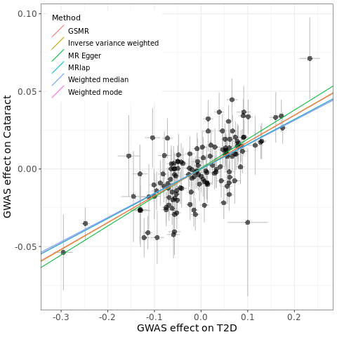

Perform MVMR if interested in mediation:

# read another exposure and iv for mvmr
df3_raw <- read.table("trait3.txt.gz", header = 1, sep = "\t")
snp_mvmr <- unlist(read.table("trait1_and_3.iv"))

# subset iv
df1 <- df1_raw %>% filter(SNP %in% snp_mvmr) %>% select(-CHR, -POS)
df2 <- df2_raw %>% filter(SNP %in% snp_mvmr) %>% select(-CHR, -POS)
df3 <- df3_raw %>% filter(SNP %in% snp_mvmr) %>% select(-CHR, -POS)

# harmonise
df1 <- df1 %>%
    mutate(id.exposure = "t2d", exposure = "t2d") %>%
    rename("pval.exposure" = "P", "effect_allele.exposure" = "A1", "other_allele.exposure" = "A2", "samplesize.exposure" = "N", "beta.exposure" = "BETA", "se.exposure" = "SE", "eaf.exposure" = "FRQ")
df3 <- df3 %>%
    mutate(id.exposure = "bmi", exposure = "bmi") %>%
    rename("pval.exposure" = "P", "effect_allele.exposure" = "A1", "other_allele.exposure" = "A2", "samplesize.exposure" = "N", "beta.exposure" = "BETA", "se.exposure" = "SE", "eaf.exposure" = "FRQ")
df2 <- df2 %>%
    mutate(id.outcome = "cataract", outcome = "cataract") %>%
    rename("pval.outcome" = "P", "effect_allele.outcome" = "A1", "other_allele.outcome" = "A2", "samplesize.outcome" = "N", "beta.outcome" = "BETA", "se.outcome" = "SE", "eaf.outcome" = "FRQ")

# run mvmr
dat <- harmonise_data(df1, df2) %>% filter(mr_keep == T)
mvdat <- mv_harmonise_data(rbind(df1, df3), df2)
res <- mv_multiple(mvdat)
res
# id.exposure exposure id.outcome  outcome nsnp    b    se   pval
#      bmi      bmi    cataract cataract   62   -0.037 0.051 4.748e-01
#      t2d      t2d    cataract cataract   88   0.179 0.016  2.506e-29

Mediation effect = 1 - direct effect (BETA estimated in MVMR) / total effect (BETA estimated in MR).
When both total effect and mediated effect align in the same direction, it indicates the presence of a mediating effect.
Environment:

Plink 1.9; R 4.2.3, with TwoSampleMR: 0.5.11, gsmr: 1.1.0, MRlap: 0.0.3.2, dplyr: 1.1.4, ggplot2: 3.5.0, ggsci: 3.0.0

LCV (Latent Causal Variable model)

LCV measures genetic causation based on GWAS summary. Demo data is two munged GWAS summary from above LDSC demo, in hg19.

Download script, LD scores, demo data:

# lcv script
wget -c https://zhanghaoyang.net/note/lcv/RunLCV.R
wget -c https://zhanghaoyang.net/note/lcv/MomentFunctions.R

# demo sumstats
wget -c https://zhanghaoyang.net/note/ldsc/trait1.sumstats.gz # bbj t2d
wget -c https://zhanghaoyang.net/note/ldsc/trait2.sumstats.gz # bbj cataract

# ld score
# LD scores (hg19). Public: https://zenodo.org/records/7768714 (EAS: 1000G_Phase3_EAS_baselineLD_v2.2_ldscores.tgz, EUR: 1000G_Phase3_ldscores.tgz). Adjust the ld paths accordingly (results approximate).
wget -c -O 1000g_ldscore_hg19.tar.gz https://zenodo.org/records/7768714/files/1000G_Phase3_ldscores.tgz # ldscore
tar -xvf 1000g_ldscore_hg19.tar.gz

Perform LCV:

# source script
source("RunLCV.R")

# load data
file_gwas1 <- "trait1.sumstats.gz"
file_gwas2 <- "trait2.sumstats.gz"
path_ld <- "1000g_ldscore_hg19/eas_ldscores/" # if your population is eur, use 'eur_w_ld_chr'

df1 <- na.omit(read.table("trait1.sumstats.gz", header = TRUE, sep = "\t", stringsAsFactors = FALSE))
df2 <- na.omit(read.table("trait2.sumstats.gz", header = TRUE, sep = "\t", stringsAsFactors = FALSE))
df3 <- data.frame()
for (chr in 1:22) {
    file <- paste0(path_ld, chr, ".l2.ldscore.gz")
    sub <- read.table(gzfile(file), header = TRUE, sep = "\t", stringsAsFactors = FALSE)
    df3 <- rbind(df3, sub)
}

# merge, sort
m <- merge(df3, df1, by = "SNP")
m2 <- merge(m, df2, by = "SNP")
data <- m2[order(m2[, "CHR"], m2[, "BP"]), ]

# qc
mismatch <- which(data$A1.x != data$A1.y, arr.ind = TRUE)
data[mismatch, ]$Z.y <- data[mismatch, ]$Z.y * -1
data[mismatch, ]$A1.y <- data[mismatch, ]$A1.x
data[mismatch, ]$A2.y <- data[mismatch, ]$A2.x

# analysis
LCV <- RunLCV(data$L2, data$Z.x, data$Z.y)
sprintf("Estimated posterior gcp=%.2f(%.2f), log10(p)=%.1f; estimated rho=%.2f(%.2f)", LCV$gcp.pm, LCV$gcp.pse, log(LCV$pval.gcpzero.2tailed) / log(10), LCV$rho.est, LCV$rho.err)

# result
# "Estimated posterior gcp=0.87(0.11), log10(p)=-8.9; estimated rho=0.55(0.12)"

SMR (Summary-data-based Mendelian Randomization)

SMR measures pleiotropic association between the expression and trait with GWAS summary.
This demo perform SMR with 49 tissues from GTEx.

# install
wget -c https://yanglab.westlake.edu.cn/software/smr/download/smr-1.3.1-linux-x86_64.zip 
unzip smr-1.3.1-linux-x86_64.zip 
cd smr-1.3.1-linux-x86_64

# download gtex eqtl
wget --recursive --level=1 --no-parent --accept-regex ".*\.zip" https://yanglab.westlake.edu.cn/data/SMR/GTEx_V8_cis_eqtl_summary.html
mv yanglab.westlake.edu.cn/data/SMR/GTEx_V8_cis_eqtl_summary ./
unzip -o 'GTEx_V8_cis_eqtl_summary/*.zip' -d 'GTEx_V8_cis_eqtl_summary/'

# download referene genome
# 1000G PLINK bfile (hg19). Public reference panel: https://zenodo.org/records/7768714 (EAS: 1000G_Phase3_EAS_plinkfiles.tgz, EUR: 1000G_Phase3_plinkfiles.tgz). Folder layout differs from this demo, adjust the bfile paths accordingly (results approximate).
wget -c -O 1000g_bfile_hg19.tar.gz https://zenodo.org/records/7768714/files/1000G_Phase3_EAS_plinkfiles.tgz
tar -xvf 1000g_bfile_hg19.tar.gz

# download demo gwas
wget -c https://zhanghaoyang.net/note/smr/trait4.txt.gz
gzip -d trait4.txt.gz

# run SMR
file_gwas=trait4.txt
path_eqtl="GTEx_V8_cis_eqtl_summary"
path_bfile="1000g_bfile_hg19/eur"
tissues=$(ls $path_eqtl | grep .zip | sed 's/\.zip//g')

for tissue in $tissues
do
  file_out="${tissue}_TO_trait4"

  if [ -e $file_out.smr ]; then continue; fi

  ./smr \
  --bfile $path_bfile \
  --gwas-summary $file_gwas \
  --beqtl-summary $path_eqtl/$tissue/$tissue \
  --diff-freq-prop 0.2 \
  --out $file_out
done

# result (e.g., Lung_TO_trait4.smr ) is like:
# probeID ProbeChr        Gene    Probe_bp        topSNP  topSNP_chr      topSNP_bp       A1      A2      Freq    b_GWAS  se_GWAS p_GWAS  b_eQTL  se_eQTL p_eQTL  b_SMR   se_SMR  p_SMR   p_HEIDI      nsnp_HEIDI
# ENSG00000186891 1       TNFRSF18        1138888 rs6603785       1       1186502 T       A       0.113497        0.0471698       0.186186        8.000000e-01    -0.226131       0.0388867   6.058973e-09     -0.208595       0.824138        8.001855e-01    7.833459e-01    3
# ENSG00000176022 1       B3GALT6 1167629 rs6697886       1       1173611 A       G       0.128834        0.0459289       0.170633        7.878000e-01    -0.145222       0.0225851       1.276171e-10 -0.316267       1.17601 7.879812e-01    8.766650e-01    4
# ...

Coloc

Coloc performs genetic colocalisation based on GWAS summary. LocusCompareR displays colocalisation. The demo is in hg19.

# load packages
libs <- c("coloc", "locuscomparer")
lapply(libs, require, character.only = TRUE)

# load demo data
file_gwas1 <- "https://zhanghaoyang.net/note/coloc/gwas1.txt"
file_gwas2 <- "https://zhanghaoyang.net/note/coloc/gwas2.txt"
gwas1 <- read.delim(file_gwas1)
gwas2 <- read.delim(file_gwas2)

# prepare list for coloc, we may also use varbeta, which is se^2
D1 <- list(pvalues = gwas1$P, snp = gwas1$SNP, position = gwas1$POS, N = gwas1$N, MAF = gwas1$FRQ)
D2 <- list(pvalues = gwas2$P, snp = gwas2$SNP, position = gwas2$POS, N = gwas2$N, MAF = gwas2$FRQ)
# define 'type' and 's' by your study
D1$type <- "cc"
D2$type <- "cc" # type="cc" for case control or type="quant" for quantitative
D1$s <- 0.33 # only for case control, proportion of cases
D2$s <- 0.33 

# coloc analysis
coloc.abf(D1, D2)
# result:
# Posterior
#        nsnps           H0           H1           H2           H3           H4
# 7.930000e+02 2.757436e-25 1.034489e-13 3.566324e-13 1.329284e-01 8.670716e-01

Plot with locuscomparer:

png("locuscomparer.png", width = 1200, height = 600, res = 150)
locuscompare(
    in_fn1 = file_gwas1, in_fn2 = file_gwas2,
    marker_col1 = "SNP", pval_col1 = "P", marker_col2 = "SNP", pval_col2 = "P",
    title1 = "GWAS1", title2 = "GWAS2"
)
dev.off()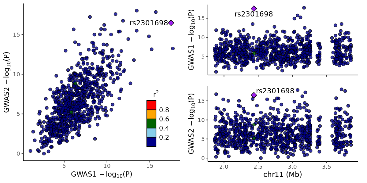

Environment:

R 4.2.3, with coloc: 5.2.3, locuscomparer: 1.0.0"

MAGMA

MAGMA performs gene-based and gene-set analysis based on GWAS summary. Gene set from MsigDB. The demo is in hg19.

# download magma script
wget -c https://ctg.cncr.nl/software/MAGMA/prog/magma_v1.10.zip # magma program (CTG Leiden)
unzip magma_v1.10.zip
mv README README_magma
# download gene set data
# MSigDB gene sets. Download msigdb_v2023.1.Hs_GMTs.tar.gz from https://www.gsea-msigdb.org/gsea/msigdb/ (free login required), then place it here.
tar -xvf msigdb_v2023.1.Hs_GMTs.tar.gz
# download bfile
# 1000G PLINK bfile (hg19). Public reference panel: https://zenodo.org/records/7768714 (EAS: 1000G_Phase3_EAS_plinkfiles.tgz, EUR: 1000G_Phase3_plinkfiles.tgz). Folder layout differs from this demo, adjust the bfile paths accordingly (results approximate).
wget -c -O 1000g_bfile_hg19.tar.gz https://zenodo.org/records/7768714/files/1000G_Phase3_EAS_plinkfiles.tgz
tar -xvf 1000g_bfile_hg19.tar.gz
# download gene pos data
wget -c https://ctg.cncr.nl/software/MAGMA/aux_files/NCBI37.3.zip # gene locations, hg19 (CTG Leiden)
unzip NCBI37.3.zip 
# download demo gwas
mkdir demo
wget -c -P demo https://zhanghaoyang.net/note/ldsc/trait1.txt.gz # demo gwas

# magma analysis
file_bfile="1000g_bfile_hg19/eas" # if your data is EUR, use "eur"
file_loc="NCBI37.3.gene.loc"
file_gwas="demo/trait1.txt.gz"; file_pval="demo/pval_file"; file_out="demo/trait1"
N="166718" # sample size

# extract pval
zcat $file_gwas  | cut -f 3,9 > $file_pval
# annotate snp
./magma \
    --annotate \
    --snp-loc $file_bfile.bim \
    --gene-loc $file_loc \
    --out $file_out

# gene-based analysis
./magma \
  --bfile $file_bfile \
  --pval $file_pval N=$N \
  --gene-annot $file_out.genes.annot \
  --out $file_out

# gene-set analysis
path_geneset="msigdb_v2023.1.Hs_GMTs/"
for i in `ls $path_geneset | grep entrez`; do 
echo $i 
./magma \
  --gene-results $file_out.genes.raw \
  --set-annot $path_geneset$i \
  --out ${file_out}_$i
done

rsidmap

rsidmap finds rsid with genomic position (CHR, POS, A1, A2) from dbsnp. dbsnp is a large dataset cover full snp.
Note: if you only work on common variants, you donn’t need ‘rsidmap’, use frq file in 1000 genomics is enough.

# download rsidmap:
git clone https://github.com/zhanghaoyang0/rsidmap.git
cd rsidmap

# download dbsnp:
url="https://ftp.ncbi.nlm.nih.gov/snp/latest_release/VCF/"
dbsnp_hg19="GCF_000001405.25"
dbsnp_hg38="GCF_000001405.40"
# for hg19
wget -c ${url}${dbsnp_hg19}.gz -P dbsnp/
wget -c ${url}${dbsnp_hg19}.gz.md5 -P dbsnp/
wget -c ${url}${dbsnp_hg19}.gz.tbi -P dbsnp/
wget -c ${url}${dbsnp_hg19}.gz.tbi.md5 -P dbsnp/
# for hg38
wget -c ${url}${dbsnp_hg38}.gz -P dbsnp/
wget -c ${url}${dbsnp_hg38}.gz.md5 -P dbsnp/
wget -c ${url}${dbsnp_hg38}.gz.tbi -P dbsnp/
wget -c ${url}${dbsnp_hg38}.gz.tbi.md5 -P dbsnp/
# check md5sum
cd dbsnp
md5sum -c ${dbsnp_hg19}.gz.md5
md5sum -c ${dbsnp_hg19}.gz.tbi.md5
md5sum -c ${dbsnp_hg38}.gz.md5
md5sum -c ${dbsnp_hg38}.gz.tbi.md5
cd ../

# rsidmap:
python ./code/rsidmap_v2.py \ 
  --build hg19 \
  --chr_col chr --pos_col pos --ref_col a2 --alt_col a1 \
  --file_gwas ./example/largedf_hg19.txt.gz \ 
  --file_out ./example/largedf_hg19_rsidmapv2.txt

# output file is like:
# CHR	POS	A1	A2	FRQ	BETA	SE	P	SNP
# X   393109  T   C   0.512	0.131	0.25	0.029	rs1603207647
# 1	10054	C	CT	0.2313	0.002	0.23	0.3121	rs1639543820
# 1	10054	CT	C	0.1213	0.042	0.12	0.0031	rs1639543798
# Y   10002   T   A   0.614	0.28	0.095	0.421	rs1226858834
# ...

Environment:

Python 3.9.6, with numpy: 1.23.1, argparse, gzip, os, time

easylift

easylift made minor efforts on LiftOver to make a lift between hg19 and hg38 easier. It omits laborious steps (i.e., prepare bed input, lift, and then map back to your files).

git clone https://github.com/zhanghaoyang0/easylift.git
cd easylift

# lift can be 'hg19tohg38' or 'hg38tohg19'
python ./code/easylift.py \
  --lift hg19tohg38 \
  --chr_col CHR --pos_col POS \
  --file_in ./example/df_hg19.txt.gz \
  --file_out ./example/df_hg19_lifted_to_hg38.txt

# The output file is like:
# CHR     POS_old A1      A2      FRQ     BETA    SE      P       POS
# 2       48543917        A       G       0.4673  0.0045  0.0088  0.6101  48316778
# 5       87461867        A       G       0.7151  0.0166  0.0096  0.08397 88166050
# 14      98165673        T       C       0.1222  -0.0325 0.014   0.02035 97699336
# 12      104289454       T       C       0.534   0.0085  0.0088  0.3322  103895676
# 11      26254654        T       C       0.0765  0.0338  0.0167  0.04256 26233107
# 4       163471758       T       C       0.612   0.0119  0.0094  0.2057  162550606

Environment:

LiftOver; Python 3.8, with pandas, argparse, os, sys, time, subprocess

Variant annotation

ANNOVAR

ANNOVAR to annotate genomic variants. First, obtain download link from here, then:

# download annovar
wget -c http://download_link/annovar.latest.tar.gz
tar zxvf annovar.latest.tar.gz
cd annovar

# download refGene
./annotate_variation.pl -buildver hg38 -downdb -webfrom annovar refGene humandb/

# (Optional) download dbNSFP if you need more information (they are LARGE):
./annotate_variation.pl -buildver hg19 -downdb -webfrom annovar dbnsfp42c humandb/
./annotate_variation.pl -buildver hg38 -downdb -webfrom annovar dbnsfp42c humandb/

# download demo vcf
wget -c https://zhanghaoyang.net/note/anno/demo.vcf # few cases from clinvar, https://ftp.ncbi.nlm.nih.gov/pub/clinvar/vcf_GRCh38/clinvar.vcf.gz

# annovar
./table_annovar.pl demo.vcf humandb/ -buildver hg38 -out demo \
-remove -protocol refGene -operation g -nastring . -vcfinput -polish

# result
cat head demo.hg38_multianno.txt 
# Chr     Start   End     Ref     Alt     Func.refGene    Gene.refGene    GeneDetail.refGene      ExonicFunc.refGene      AAChange.refGene        Otherinfo1      Otherinfo2      Otherinfo3      Otherinfo4    Otherinfo5      Otherinfo6      Otherinfo7      Otherinfo8      Otherinfo9      Otherinfo10     Otherinfo11
# 1       69134   69134   A       G       exonic  OR4F5   .       nonsynonymous SNV       OR4F5:NM_001005484:exon1:c.A44G:p.E15G  .       .       .       1       69134   2205837 A       G       .    .ALLELEID=2193183;CLNDISDB=MeSH:D030342,MedGen:C0950123;CLNDN=Inborn_genetic_diseases;CLNHGVS=NC_000001.11:g.69134A>G;CLNREVSTAT=criteria_provided,_single_submitter;CLNSIG=Likely_benign;CLNVC=single_nucleotide_variant;CLNVCSO=SO:0001483;GENEINFO=OR4F5:79501;MC=SO:0001583|missense_variant;ORIGIN=1
# 1       69581   69581   C       G       exonic  OR4F5   .       nonsynonymous SNV       OR4F5:NM_001005484:exon1:c.C491G:p.P164R        .       .       .       1       69581   2252161 C       G    ..       ALLELEID=2238986;CLNDISDB=MeSH:D030342,MedGen:C0950123;CLNDN=Inborn_genetic_diseases;CLNHGVS=NC_000001.11:g.69581C>G;CLNREVSTAT=criteria_provided,_single_submitter;CLNSIG=Uncertain_significance;CLNVC=single_nucleotide_variant;CLNVCSO=SO:0001483;GENEINFO=OR4F5:79501;MC=SO:0001583|missense_variant;ORIGIN=1
# ...

# if you need dbNSFP
./table_annovar.pl demo.vcf humandb/ -buildver hg38 -out demo \
  -remove -protocol refGene,dbnsfp42c -operation g.f -nastring . -vcfinput -polish

easyanno made minor efforts on ANNOVAR to make annotate easier on format like GWAS summary.

# download easyanno
git clone https://github.com/zhanghaoyang0/easyanno.git
cd easyanno

# If annovar/ is not in your easyanno folder, add a soft link:
ln -s path_of_your_annovar ./
# check if it link correctly
ls annovar/ # you will see the scripts and data

# demo:
python ./code/easyanno.py \
  --build hg19 \
  --only_find_gene F \
  --anno_dbnsfp F \
  --chr_col CHR --pos_col POS --ref_col A2 --alt_col A1 \
  --file_in ./example/df_hg19.txt \
  --file_out ./example/df_hg19_annoed.txt

# The output file is like:
# CHR     POS     A1      A2      FRQ     BETA    SE      P       Func.refGene    Gene.refGene
# 2       48543917        A       G       0.4673  0.0045  0.0088  0.6101  intronic        FOXN2
# 5       87461867        A       G       0.7151  0.0166  0.0096  0.08397 intergenic      LINC02488;TMEM161B
# 14      98165673        T       C       0.1222  -0.0325 0.014   0.02035 intergenic      LINC02291;LINC02312
# 12      104289454       T       C       0.534   0.0085  0.0088  0.3322  ncRNA_intronic  TTC41P
# 11      26254654        T       C       0.0765  0.0338  0.0167  0.04256 intronic        ANO3
# 4       163471758       T       C       0.612   0.0119  0.0094  0.2057  intergenic      FSTL5;MIR4454

# If you set only_find_gene as F, you get more information in refgene database:
# If you set anno_dbnsfp as T, you get much more information in refgene and dbnsfp database.

Environment (for easyanno):

Python 3.9.6, with pandas: 1.4.3, numpy: 1.20.3, argparse, os, sys, time, subprocess

VEP

VEP to annotate genomic variant.

# download vep cache data
wget -c http://ftp.ensembl.org/pub/release-111/variation/indexed_vep_cache/homo_sapiens_vep_111_GRCh38.tar.gz
wget -c http://ftp.ensembl.org/pub/release-111/variation/indexed_vep_cache/homo_sapiens_refseq_vep_111_GRCh38.tar.gz
tar xvf *.tar.gz

# download fasta
mkdir genome
wget -c -P genome https://genvisis.umn.edu/rsrc/Genome/hg38/hg38.fa
wget -c -P genome https://genvisis.umn.edu/rsrc/Genome/hg38/hg38.fa.fai

# download demo vcf
wget -c https://zhanghaoyang.net/note/anno/demo.vcf # few cases from clinvar, https://ftp.ncbi.nlm.nih.gov/pub/clinvar/vcf_GRCh38/clinvar.vcf.gz

# pull and run docker
docker pull ensemblorg/ensembl-vep
docker run -t -i -v ./:/data ensemblorg/ensembl-vep

# vep (in docker)
vep --cache_version 111 --offline --assembly GRCh38 --format vcf \
    --mane_select --input_file demo.vcf  --output_file output.vcf 

# result
  cat output.vcf
# Uploaded_variation     Location        Allele  Gene    Feature Feature_type    Consequence     cDNA_position   CDS_position    Protein_position        Amino_acids     Codons  Existing_variation   Extra
# 2205837 1:69134 G       ENSG00000186092 ENST00000641515 Transcript      missense_variant        167     107     36      E/G     gAa/gGa -       IMPACT=MODERATE;STRAND=1;MANE_SELECT=NM_001005484.2
# 2252161 1:69581 G       ENSG00000186092 ENST00000641515 Transcript      missense_variant        614     554     185     P/R     cCc/cGc -       IMPACT=MODERATE;STRAND=1;MANE_SELECT=NM_001005484.2
# ...

# more result
fields='Uploaded_variation,SYMBOL,Gene,Location,REF_ALLELE,Allele,Consequence,VARIANT_CLASS,HGVSc,HGVSp,Feature,IMPACT,CANONICAL'
vep \
  --fields $fields \
  --cache_version 111 --fasta genome/hg38.fa --assembly GRCh38 --species homo_sapiens \
  --refseq --offline --variant_class --hgvs --symbol --canonical --show_ref_allele --tab --no_stat --force_overwrite --no_headers \
  --shift_3prime 1 \
  --input_data "1 69134 69134 A/G +" \
  --output_file STDOUT 
# result
# 1_69134_A/G     OR4F5   79501   1:69134 A    G    missense_variant    SNV  NM_001005484.2:c.107A>G NP_001005484.2:p.Glu36Gly  NM_001005484.2  MODERATE  YES

TransVar

TransVar to annotate genomic, protein, cDNA variant.

# download fasta
mkdir genome
wget -c -P genome https://genvisis.umn.edu/rsrc/Genome/hg38/hg38.fa
wget -c -P genome https://genvisis.umn.edu/rsrc/Genome/hg38/hg38.fa.fai

## annotate genomic variant
docker run -v ./genome/:/ref zhouwanding/transvar:latest  \
    transvar ganno -i 'chr3:g.178936091_178936192' --ensembl --reference /ref/hg38.fa
# result
# input   transcript      gene    strand  coordinates(gDNA/cDNA/protein)  region  info
# chr3:g.178936091_178936192      .       .       .       chr3:g.178936091_178936192/./.  inside_[intergenic_between_KCNMB2-AS1(75686_bp_upstream)_and_ZMAT3(81031_bp_downstream)]      .

## annotate cdna variant
docker run -v ./genome/:/ref zhouwanding/transvar:latest  \
    transvar canno -i 'PIK3CA:c.1633G>A' --ensembl --reference /ref/hg38.fa
# result
# input   transcript      gene    strand  coordinates(gDNA/cDNA/protein)  region  info
# PIK3CA:c.1633G>A        ENST00000263967 (protein_coding)        PIK3CA  +       chr3:g.179218303G>A/c.1633G>A/p.E545K   inside_[cds_in_exon_10] CSQN=Missense;reference_codon=GAG;alternative_codon=AAG;aliases=ENSP00000263967;source=Ensembl
# PIK3CA:c.1633G>A        ENST00000643187 (protein_coding)        PIK3CA  +       chr3:g.179218303G>A/c.1633G>A/p.E545K   inside_[cds_in_exon_10] CSQN=Missense;reference_codon=GAG;alternative_codon=AAG;aliases=ENSP00000493507;source=Ensembl

## annotate protein variant
docker run -v ./genome/:/ref zhouwanding/transvar:latest  \
    transvar panno -i COL1A2:p.E545K --ensembl --reference /ref/hg38.fa
# result
# input   transcript      gene    strand  coordinates(gDNA/cDNA/protein)  region  info
# COL1A2:p.E545K  ENST00000297268 (protein_coding)        COL1A2  +       chr7:g.94413915G>A/c.1633G>A/p.E545K    inside_[cds_in_exon_28] CSQN=Missense;reference_codon=GAA;candidate_codons=AAG,AAA;candidate_mnv_variants=chr7:g.94413915_94413917delGAAinsAAG;aliases=ENSP00000297268;source=Ensembl

BLAST

BLAST finds regions of similarity between biological sequences.

# download blast
wget -c https://ftp.ncbi.nlm.nih.gov/blast/executables/blast+/LATEST/ncbi-blast-2.16.0+-x64-linux.tar.gz
tar -zxvf ncbi-blast-2.16.0+-x64-linux.tar.gz

# download ref genome fasta 
wget -c -P genome https://genvisis.umn.edu/rsrc/Genome/hg38/hg38.fa
wget -c -P genome https://genvisis.umn.edu/rsrc/Genome/hg38/hg38.fa.fai

# make blast db
file_fasta_ref="hg38.fa"
ncbi-blast-2.16.0+/bin/makeblastdb -in $file_fasta_ref -out $file_fasta_ref -dbtype nucl

# demo, align a short seq
echo -e ">seq\nCGAGTAGGGGCTGGTGACAG" > fasta_query

ncbi-blast-2.16.0+/bin/blastn  \
  -db  $file_fasta_ref \
  -task blastn-short -evalue 1 \
  -query fasta_query \
  -out result -outfmt 0

# result is like:
# ...
# Sequences producing significant alignments:                          (Bits)  Value
# chr2 AC:CM000664.2 gi:568336022 LN:242193529 rl:Chromosome M5:f98...  40.1    0.008
# chr1 AC:CM000663.2 gi:568336023 LN:248956422 rl:Chromosome M5:6ae...  34.2    0.49 
# ...
# Score = 40.1 bits (20),  Expect = 0.008
# Identities = 20/20 (100%), Gaps = 0/20 (0%)
# Strand=Plus/Plus
# Query  1         CGAGTAGGGGCTGGTGACAG  20
#                 ||||||||||||||||||||
# Sbjct  47476492  CGAGTAGGGGCTGGTGACAG  47476511

Genetic Analysis

Table of Contents

GWAS

MTAG (Multi-Trait Analysis of GWAS)

Genetic correlation

LDSC (LD Score Regression)

HDL (High-Definition Likelihood)

LAVA (Local Analysis of Variant Association)

GPA (Genetic analysis incorporating Pleiotropy and Annotation)

Genetic causality

MR (Mendelian randomization)

LCV (Latent Causal Variable model)

SMR (Summary-data-based Mendelian Randomization)

Coloc

MAGMA

rsidmap

easylift

Variant annotation

ANNOVAR

VEP

TransVar

BLAST